USRP-1 has two fpga images :
One with half-band filters and another one without half-and filters.
The fpga file with half-band filter is
usrp1_fpga.rbf located in /usr/local/share/uhd/images
USRP1 cannot achieve decimations below 8 when the half-band filter is present.
This means you cant get samples more than 8 MSPS in the CPU when the half-bad filters are present because actual rate at which CPU receives samples is adc_rate/decim_rate i.e. 64MSPS/decim_rate , so if decim_rate >=8
this implies samples per sec to CPU <= 8MHz and hence we wont be able to see more than 8MHz
The another image i.e. usrp1_fpga_4rx.rbf file is a special FPGA image without RX half-band filters.
To load this image, set the device address key/value pair: fpga=usrp1_fpga_4rx.rbf
uhd_fft -a "fpga=usrp1_fpga_4rx.rbf"
Even after using this fpga image you wont get samples more than 16MSPS to the CPU
If you try to go above , it will get back to 16MSPS only,
So this means no decimation less than 4 is possible in any of the current FPGA images.
** Keep in mind that if you use this image then there is no low pass
filtering by the half-band filter. Low pass filtering is essentially
required after decimation. So in this case you have to do low pass
filtering in software by yourself.
** uhd set_samp_rate never fails; always falls back to closest requested
** If the USRP DDC decimation rate is X. The CIC filter response
(decimation =Y ), HBF response (decimation =Z) and cascaded CIC + HBF
(total decimation =Y*Z ) i.e. X is actually Y*Z ... Since DDC is implemented with CIC and half-band filters !!
** But for the another image i.e. without half-band filter, the total decimation = Y only
** CIC decimator is a fourth order filter here
Details about CIC decimator can be found in
/fpga/usrp1/sdr_lib/cic_decim.v
** Half-band filter is 31 tap
The coefficients of the Half-band are symmetric, and with the exception of the middle tap, every other coefficient is zero. The middle section of taps looks like this:
..., -1468, 0, 2950, 0, -6158, 0, 20585, 32768, 20585, 0, -6158, 0, 2950, 0, -1468, |
middle tap -------+
Details about its implementation can be found in
/fpga/usrp1/sdr_lib/hb/halfband_decim.v
~~~~~~~~~~~~~~~~~~~~~~~~~~~~~~~~~~~~~~~~~~~~~~~~~~~
One interesting discussion :
Reference :
http://gnuradio.4.n7.nabble.com/Disabling-the-USRP-FPGA-HBF-tt12603.html
Is there away to disable (or bypass) the USRP FPGA DDC half band
filter? I want to get the samples directly from the CIC decimation
filter and do the low pass filtering by software. I developed a MATLAB
based professional 100KHz bandwidth digital down converter as shown in
the attached m file. I want to test this design in USRP. In the mean
time, I cannot do this because I don't have access to the CIC output
samples because of the HBF.
Waiting for your help, thank you.
Firas.
If receive only is OK, you can use the "fpga=usrp1_fpga_4rx.rbf" configuration
Eric
~~~~~~~~~~~~~~~~~~~~~~~~~~~~~~~~~~~~~~~~~~~~~~~~~
A very nice discussion about frequency response of the various filters involved in the DDC stages.
Reference :
http://gnuradio.4.n7.nabble.com/wise-big-block-interleaving-in-GNURadio-tt12573.html#a12576
USRP CIC Frequency Response :

USRP CIC Frequency Response Zoomed :

USRP half-band Filter Frequency Response :

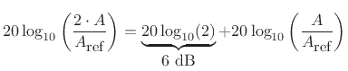


 which is
proportional to
which is
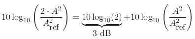
proportional to  is said to ``fall off'' (or ``roll off'') at the
rate of
is said to ``fall off'' (or ``roll off'') at the
rate of  dB per decade. That is, for every factor of
  in
in  (every ``decade''), the amplitude drops
 dB per octave. That is, for every factor of
  in
in 

